Recent Weights Ensembel Techniques in Deep Learning

Disclaimer: To write this blog I read several blogs from Medium authors Max Pechyonkin and Vitaly Bushaev. Thanks to them and the relevant arxiv papers. Also I referto this beautiful blog.

Summary

Ensemble is common way for kagglers to get the best performance by commbining the performances of different models. In practice, serveral kagglers share their own best-performance models to ensemble them to a final best one. Xgboost and other boost methods are thus becoming the secret weapons for the final round kagglers. However, it is difficult to train so many models in research to boost the performance by serveral points or so for the GPU computing is quite expensive. We still want to take the advantages of ensemble. So the first weights ensemble comes. Before that, let’s look at some relevant techniques in training.

Before start

Geometric Views of weights

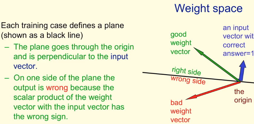
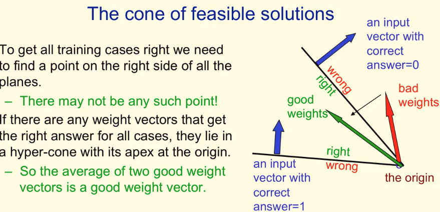
At any point of training. The network with the weights in it, or the solution we have so far can be viewd as a vector while the inputs can be viewd as a plane. Our goal is to find such “good” vectors that can seperate the input planes, or find vectors which multiplies with the input vectors can lead to positive sign of the plane. The solution space is concave, thus two such good solutions can combine to make a new good solution. This is a base knowledge that we can emsemble our weights to get a better one.

Left: In weight space, every input is a plane and every set of weights(solution) is a vector(point) in the space. Right: sum of two good solutions is also a good solution due tot concave properties.

Wide-Sharpe-Minimum

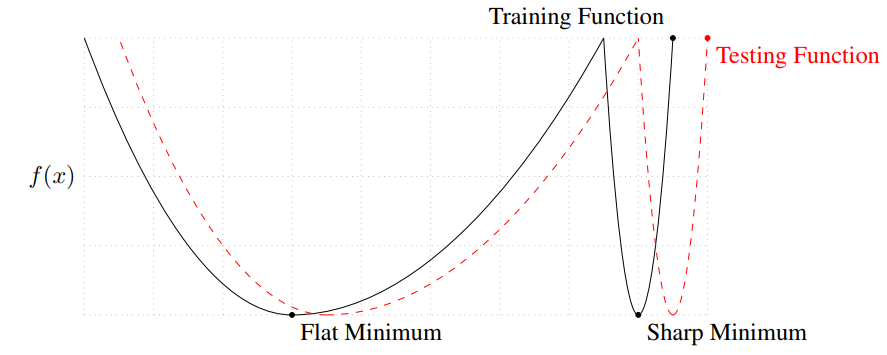
As in the paper ON LARGE-BATCH TRAINING FOR DEEP LEARNING:GENERALIZATION GAP AND SHARP MINIMA (I should have read it earlier!). The ability of generation from training set to test set is viewed as the problem whether the minimum is sharpe or wide. Just as the figure below, the good(well generalized) solution should be the wider ones.

The dotted line is the test error function while the real line is the train error function. The error function is somewhat divergent with the train error function. Intuitively, the wide local minimum of training loss can also achive good result in test error function while there is big gap between the training and test loss in the sharp local minimum. Which shows that the wide local minimum can generalize better and is the solution we want.

Learning rate schedule

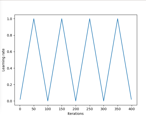
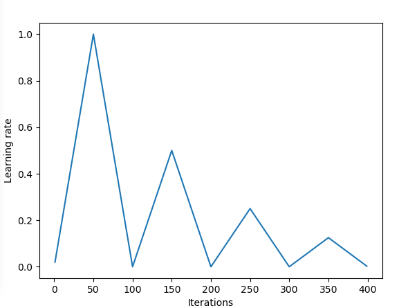
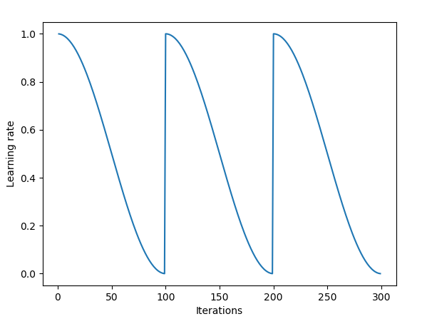
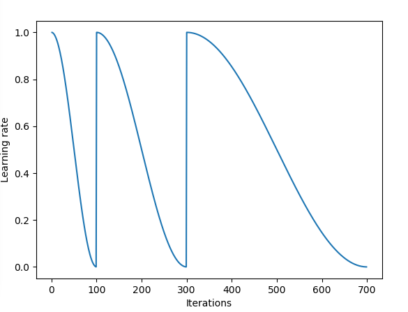
You can refer to this blog for more details about this part. We usually use constant learning rates during training. But the problem is that such constant lr can lead to traing stuck at the saddle point. In Leslie N. Smith’s “triangular” learning rate paper, a triangle shape learning rate is proposed to alleviate the problem. Inspired by this, cosine lr up and down also comes out and proves to be more effective.

Left: In a cycle(a fixed number of iterations), lr goes from low to high and returns to the original low point. Right: “triangle” learing rate v2, the high points reduces to its half as cycle number goes on.

Left: In a cycle(a fixed number of iterations), lr goes high to low in a cosine rate and cycles again. Right: Cycles like left one except the time period of the cycle doubles.

Snapshot Ensembling

Ensemble weights of different local minimums

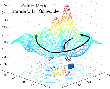
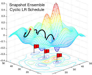
Unlike other model ensemble methods. The author comes up with the creative idea of increasing the learning rate to escape the current local minimum instead of training from start over to get another minum. Thus the training cost is cut down sharply. I followed the Keras code implementation to get a 71.04, 71.78 and 72.24 accuracy on the CIFAR100 dataset using single best model, non-weighted ensemble model, weighted ensemble model respectively.

Left: Single best model falls into a local minimum. Right: Snapshot ensemble restarts from the minimum to find more minimum by increasing the lr when stuck.

Fast Geometric Ensembling

Ensemble minimas on the the path

The authors found that there exists path between the local minimas, on this path the loss stays low. Therefore it can take smaller steps and shorter cycles to find different enough minimas to ensemble with, and produce better results than the Snapshot Ensembling.

Left: By intuition, we need to find a path to get to another minima which crosses a high loss region. Middle,Right: However the author finds that there is a path directly connects these local minimas. On this path the loss stays low and it takes smaller steps and shorter cycles.

Stochastic Weight Averaging (SWA)

Only two set of weights to ensemble

The Author observes that after every cycle, the solution stops at the boarder of the “real global minima”, so intuitively just average these solution weights. In practice, the paper gives a formula to let two set of weights to update the averaging. And at last one final weight is used to inference.

Left: W1, W2 and W3 represent 3 independently trained networks, Wswa is the average of them. Middle: Wswa provides superior performance on the test set as compared to SGD. Right: Note that even though Wswa shows worse loss during training, it generalizes better.

\[ \frac{w_{SWA} + n_{models} + w}{n_{models}+1} \to w_{SWA}. \]

This is the formula to update the average after get a new minima

Update on Feb,23: the same group put a new paper “SWAG” “A Simple Baseline for Bayesian Uncertainty in Deep Learning”, pdf link

to be continued….